
Phytopatometry in R with the package pliman
Tiago Olivoto
2025-08-02
Source:vignettes/phytopatometry.Rmd
phytopatometry.RmdSingle images
library(pliman)
#> ╭ Welcome to pliman version "3.1.0"! ──────────────────────────────╮
#> │                                                                  │
#> │   Developed collaboratively by NEPEM <https://nepemufsc.com>     │
#> │   Group lead: Prof. Tiago Olivoto                                │
#> │   For citation, type `citation('pliman')`                        │
#> │   We welcome your feedback and suggestions!                      │
#> │                                                                  │
#> ╰────────────── Simplifying high-throughput plant phenotyping in R ╯
# set the path directory
path_soy <- "https://raw.githubusercontent.com/TiagoOlivoto/images/master/pliman"
# import images
img <- image_import("leaf.jpg", path = path_soy)
healthy <- image_import("healthy.jpg", path = path_soy)
symptoms <- image_import("sympt.jpg", path = path_soy)
background <- image_import("back.jpg", path = path_soy)
image_combine(img, healthy, symptoms, background, ncol = 4)
Image palettes
Sample palettes can be created by manually sampling small areas of
representative images and producing a composite image that represents
each of the desired classes (background, healthy, and symptomatic
tissues). Another approach is to use the image_palette()
function to generate sample color palettes.
pals <- image_palette(img, npal = 8, return_pal = TRUE)
#> ℹ Processing a single image. Please, wait.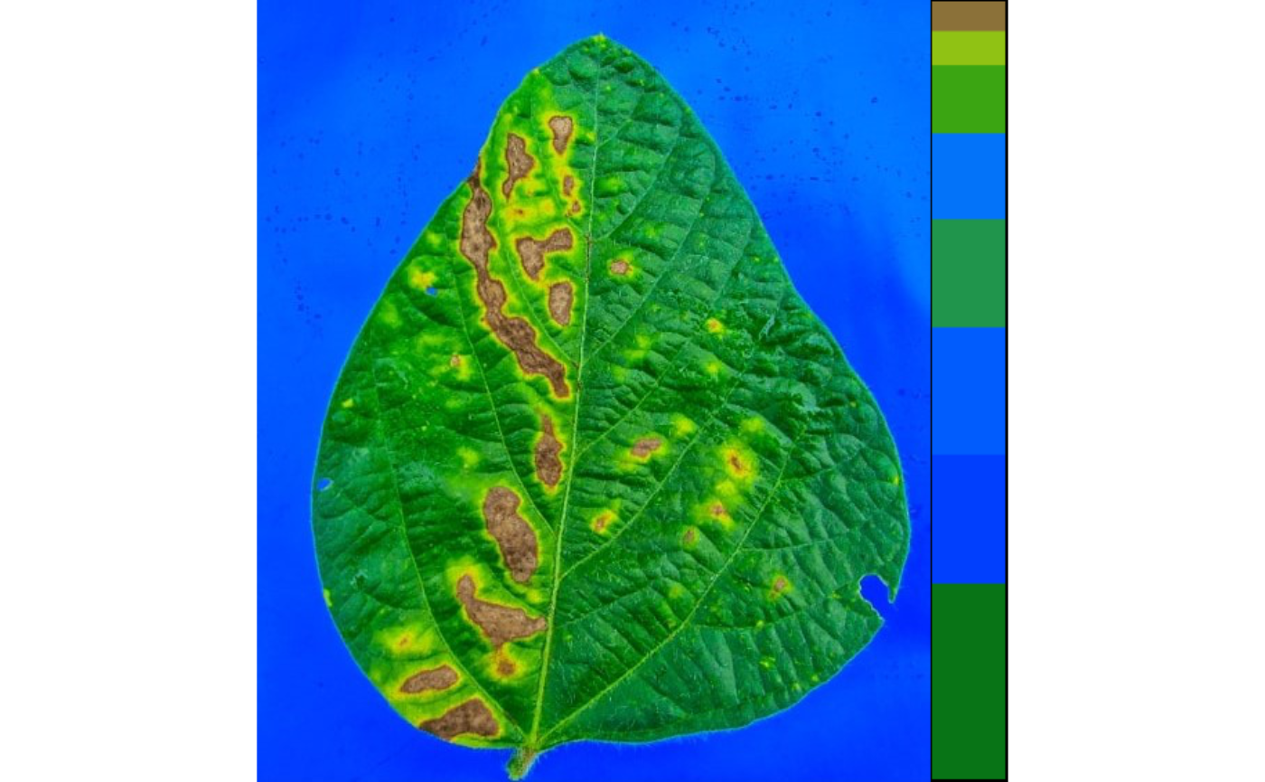
#> ✔ Image Successfully analyzed! [937ms]
image_combine(pals$palette_list, ncol = 4)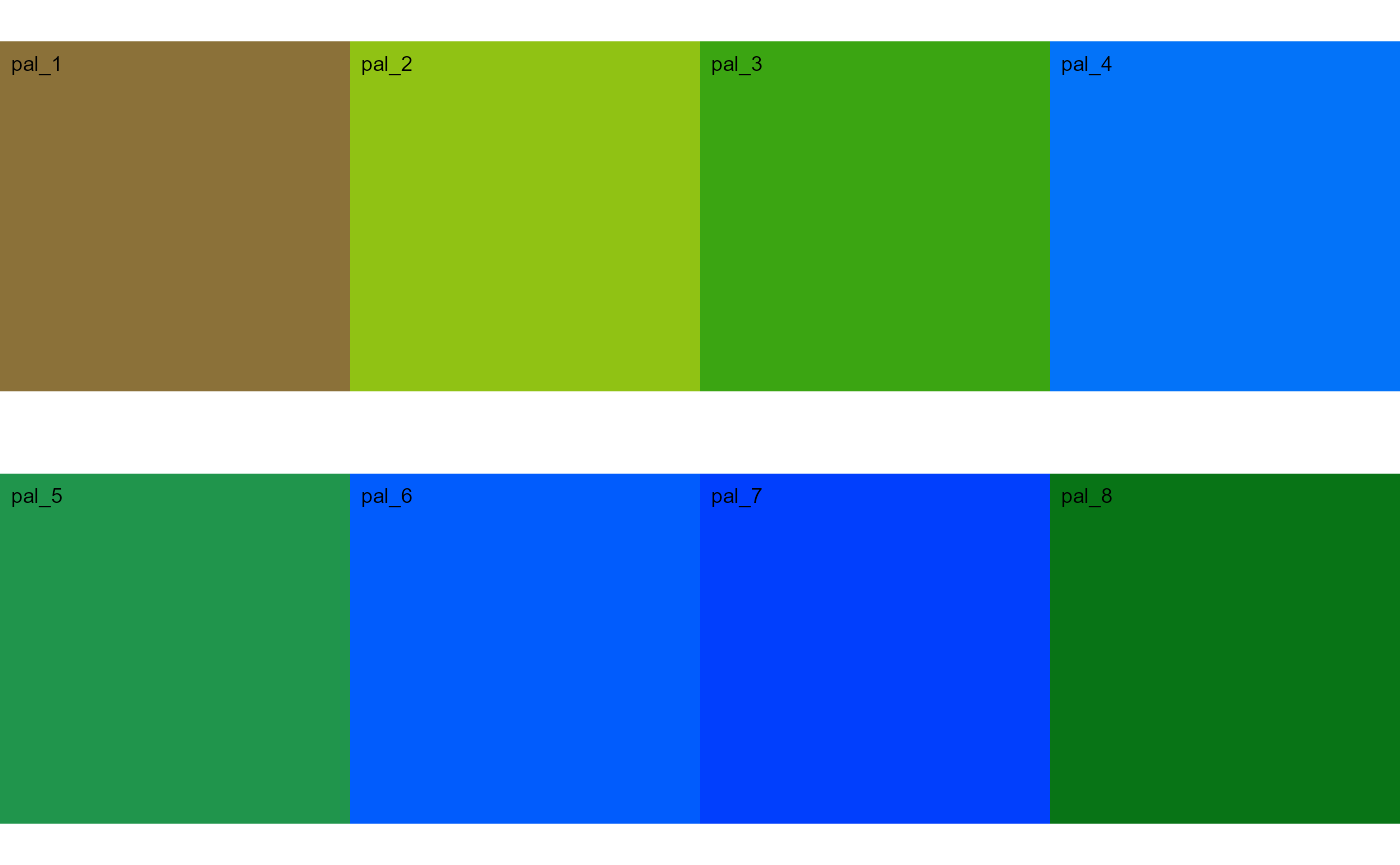
# default settings
res <-
  measure_disease(img = img,
                  img_healthy = healthy,
                  img_symptoms = symptoms,
                  img_background = background)
#> ℹ Processing a single image. Please, wait.
#> ✔ Image Successfully analyzed! [940ms]
res$severity
#>    healthy symptomatic
#> 1 89.41419    10.58581
Alternatively, users can create a mask instead of displaying the original image.
# create a personalized mask
res2 <-
  measure_disease(img = img,
                  img_healthy = healthy,
                  img_symptoms = symptoms,
                  img_background = background,
                  show_original = FALSE, # create a mask
                  show_contour = FALSE, # hide the contour line
                  col_background = "white", # default
                  col_lesions = "red", # default
                  col_leaf = "green") # default
#> ℹ Processing a single image. Please, wait.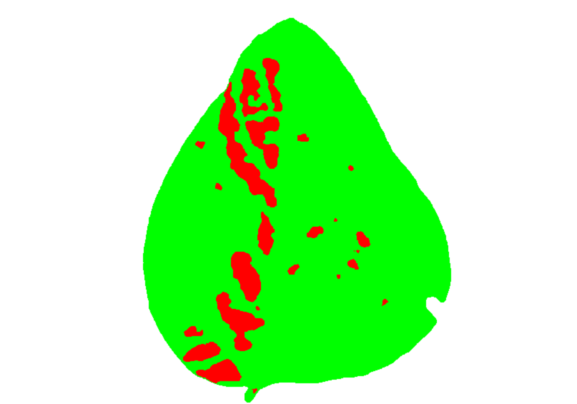
#> ✔ Image Successfully analyzed! [1.2s]


res2$severity
#>    healthy symptomatic
#> 1 89.12594    10.87406
Variations in image palettes
The results may vary depending on how the palettes are chosen and are subjective due to the researcher’s experience. In the following example, I present a second variation in the color palettes, where only the necrotic area is assumed to be the diseased tissue. Therefore, the symptomatic area will be smaller than in the previous example.
# import images
healthy2 <- image_import("healthy2.jpg", path = path_soy)
symptoms2 <- image_import("sympt2.jpg", path = path_soy)
background2 <- image_import("back2.jpg", path = path_soy)
image_combine(healthy2, symptoms2, background2, ncol = 3)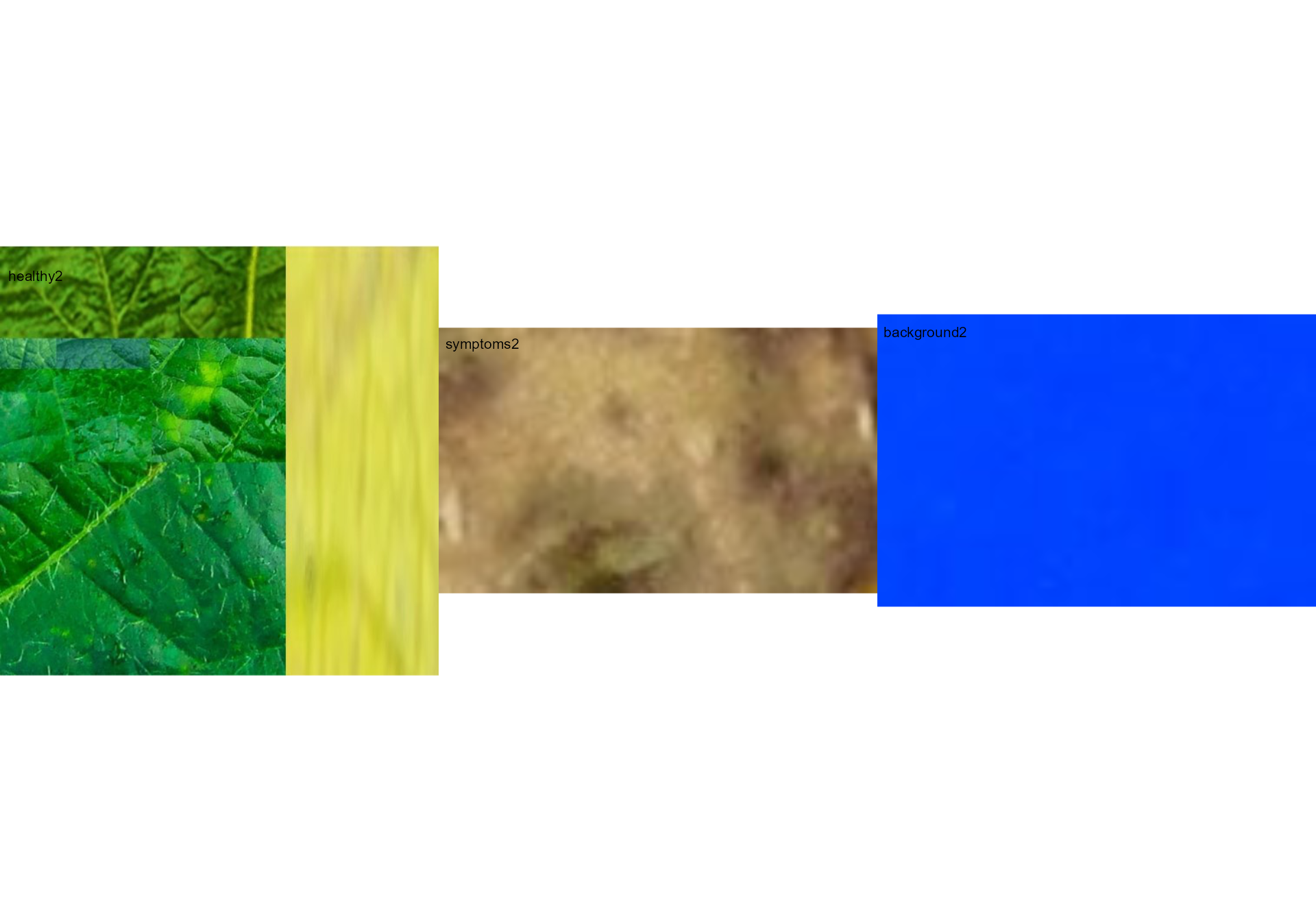
res3 <-
  measure_disease(img = img,
                  img_healthy = healthy2,
                  img_symptoms = symptoms2,
                  img_background = background2)
#> ℹ Processing a single image. Please, wait.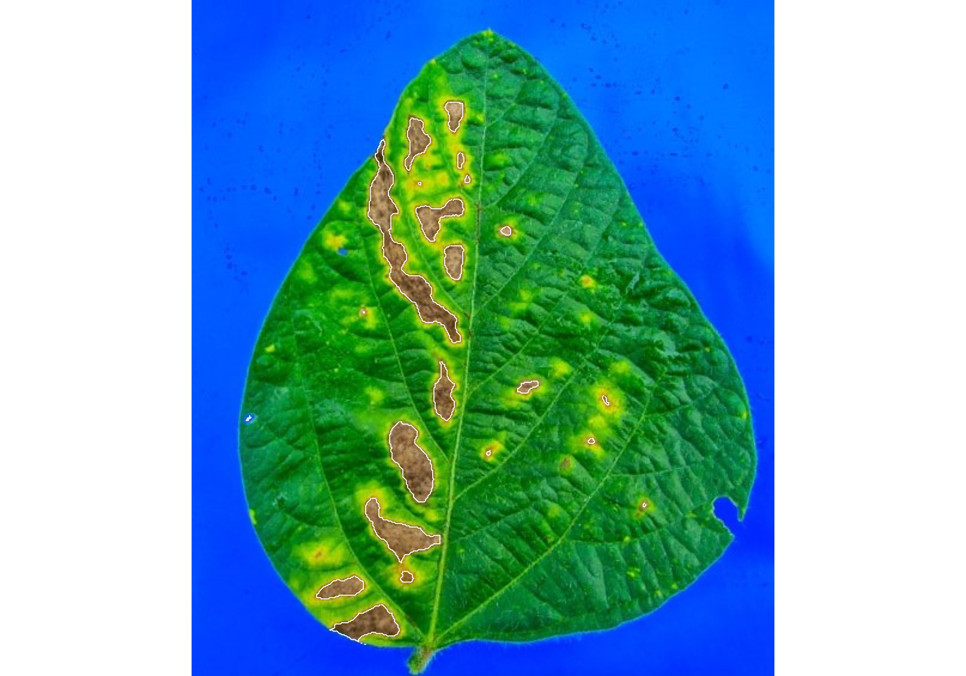
#> ✔ Image Successfully analyzed! [920ms]
res3$severity
#>    healthy symptomatic
#> 1 93.70262    6.297382
Lesion features
res4 <-
  measure_disease(img = img,
                  img_healthy = healthy,
                  img_symptoms = symptoms,
                  img_background = background,
                  show_features = TRUE,
                  marker = "area")
#> ℹ Processing a single image. Please, wait.
#> ✔ Image Successfully analyzed! [824ms]
res4$shape
#>    id       mx       my area perimeter radius_mean radius_min radius_max
#> 1   1 221.3165 113.4328 1031 199.61017   22.385350  0.5540181  39.303781
#> 2   2 189.7396 129.3218 1325 252.96551   20.485982  1.7037877  38.799639
#> 3   3 177.8770 213.1486 3732 477.54625   50.090770  1.0902575  94.465812
#> 4   4 209.8401 193.4394 1828 255.48023   23.996324  1.5966013  42.398981
#> 5   5 263.2815 192.5938  142  45.48528    6.358657  4.4175177   8.445866
#> 6   6 119.5743 201.5020  100  36.79899    5.228316  3.3866985   6.858005
#> 8   8 144.9601 260.6239   73  30.55635    4.455795  2.9165344   5.893080
#> 9   9 210.8900 328.2504  927 149.46804   18.429302  7.4482266  30.835115
#> 11 11 280.3464 323.9627  271  64.69848    9.081303  5.3468492  12.656433
#> 12 12 347.0344 334.8566  292  67.11270    9.362710  5.4703505  12.763533
#> 15 15 183.8025 384.5571 1873 192.19596   24.893179 12.8303409  38.668805
#> 16 16 333.2704 369.1409  154  47.04163    6.653785  4.2700345   9.079004
#> 17 17 249.6548 376.3188  148  47.45584    6.708013  3.3705340   9.715189
#> 19 19 172.3723 449.2197 2254 281.35029   28.651469 12.6030915  47.507444
#> 23 23 109.2006 464.1006  267  72.69848    8.948391  3.5339436  13.739762
#> 24 24 122.6708 492.3326  941 134.63961   17.881356  9.6681628  28.326603
#> 25 25 149.0925 520.2243 1291 164.53911   21.110835 11.0842927  32.910027
#>     radius_sd diam_mean  diam_min  diam_max  maj_axis  min_axis    length
#> 1  11.2387019  44.77070  1.108036  78.60756 24.156267  6.570653  76.56860
#> 2   9.0009555  40.97196  3.407575  77.59928 19.673400 10.643388  66.44392
#> 3  25.4804934 100.18154  2.180515 188.93162 54.673996 12.943501 185.16314
#> 4  10.1528815  47.99265  3.193203  84.79796 22.384645 13.318187  73.96521
#> 5   1.2039912  12.71731  8.835035  16.89173  5.315765  3.686707  15.63089
#> 6   1.0354915  10.45663  6.773397  13.71601  4.183570  3.297236  12.95079
#> 8   0.8150592   8.91159  5.833069  11.78616  3.669126  2.651668  11.13429
#> 9   6.4491505  36.85860 14.896453  61.67023 17.899320  7.779947  60.30752
#> 11  2.0643425  18.16261 10.693698  25.31287  7.932278  4.871938  24.62782
#> 12  2.0362289  18.72542 10.940701  25.52707  8.065112  5.166262  25.00000
#> 15  7.4860986  49.78636 25.660682  77.33761 22.941735 12.208977  73.66650
#> 16  1.3897121  13.30757  8.540069  18.15801  5.608257  3.834645  17.24808
#> 17  1.7199164  13.41603  6.741068  19.43038  5.985572  3.472223  18.38034
#> 19  9.8999251  57.30294 25.206183  95.01489 26.392194 14.898455  87.42711
#> 23  2.8680352  17.89678  7.067887  27.47952  8.113634  4.726704  26.00297
#> 24  5.5775852  35.76271 19.336326  56.65321 16.806900  8.253155  54.07933
#> 25  6.0422992  42.22167 22.168585  65.82005 19.273430 10.509904  62.91489
#>        width
#> 1  22.625870
#> 2  37.438748
#> 3  46.019408
#> 4  46.409925
#> 5  10.656511
#> 6   9.701347
#> 8   7.941107
#> 9  23.673758
#> 11 14.817363
#> 12 15.199658
#> 15 34.959699
#> 16 11.608204
#> 17 10.650662
#> 19 54.480476
#> 23 14.011945
#> 24 22.456618
#> 25 32.794445
res4$statistics
#>        stat      value
#> 1         n    17.0000
#> 2  min_area    73.0000
#> 3 mean_area   979.3529
#> 4  max_area  3732.0000
#> 5   sd_area  1002.9329
#> 6  sum_area 16649.0000
Interactive disease measurements
An alternative approach to measuring disease percentage is available
through the measure_disease_iter() function. This function
offers an interactive interface that empowers users to manually select
sample colors directly from the image. By doing so, it provides a highly
customizable analysis method.
One advantage of using measure_disease_iter() is the
ability to utilize the “mapview” viewer, which enhances the analysis
process by offering zoom-in options. This feature allows users to
closely examine specific areas of the image, enabling detailed
inspection and accurate disease measurement.
img <- image_pliman("sev_leaf.jpg", plot = TRUE)
measure_disease_iter(img, viewer = "mapview")