Introduction
The two main function families in pliman —shapefile_*()
and mosaic_*()— serve as the foundation for high-throughput
phenotyping (HTP) analysis. The shapefile_build() function
is central for constructing shapefiles, offering customizable layouts
and export options that allow users to tailor shapefiles to diverse
experimental designs and field layouts, enhancing the relevance and
reproducibility of the data collected.
Following shapefile creation, the mosaic_*() family is
pivotal for performing mosaic analysis —a process that includes
calculating vegetation indices, segmenting plant canopies, and
visualizing plant-level data. The mosaic_analyze()
function, in particular, automates the extraction of detailed phenotypic
information, making it easy to capture metrics on plant health, spatial
distribution, and structure across fields. Through practical examples,
users learn to leverage this function for automating plant-level data
extraction, thus boosting the efficiency and depth of HTP workflows.
All shapefiles and orthomosaics used in this vignette are publicly available here, ensuring reproducibility and allowing users to follow along with each example. Since the data is accessed remotely, an active internet connection is required to run the examples. Alternatively, you can download the entire repository and modify the code to import the files from a local source, making it more convenient for offline use and adaptable to different working environments.
R packages
library(dplyr)
#>
#> Attaching package: 'dplyr'
#> The following objects are masked from 'package:stats':
#>
#> filter, lag
#> The following objects are masked from 'package:base':
#>
#> intersect, setdiff, setequal, union
library(ggplot2)
library(pliman)
#> ╭ Welcome to pliman version "3.1.0"! ──────────────────────────────╮
#> │ │
#> │ Developed collaboratively by NEPEM <https://nepemufsc.com> │
#> │ Group lead: Prof. Tiago Olivoto │
#> │ For citation, type `citation('pliman')` │
#> │ We welcome your feedback and suggestions! │
#> │ │
#> ╰────────────── Simplifying high-throughput plant phenotyping in R ╯
#>
#> Attaching package: 'pliman'
#> The following object is masked from 'package:dplyr':
#>
#> %>%Shapefiles
Building
Shapefiles are a widely used format in geographic information systems (GIS) for representing vector data such as points, lines, and polygons. They are essential in spatial analysis and can store information about geographical features and their attributes. There are three main geometry types.
- Points: Represent specific locations (e.g., control points, cities).
- Lines: Represent linear features (e.g., roads, rivers).
- Polygons: Represent areas (e.g., boundaries of regions or land parcels).
Below, we explore how theshapefile_build() function
works for constructing shapefiles. By default, calling
shapefile_build(mosaic, ...) allows the creation of either
rectangular grids (defined by rows and columns) or custom, free-form
shapes, providing flexibility for different experimental designs.
To create a rectangular grid, you define the corners of your region
of interest (ROI) in this sequence: top left → top right →
bottom right → bottom left → back to top left to close the
polygon. If more than four points are provided, the function will
interpret them as vertices of a free-form shape, constructing a
customized polygon that precisely fits your specified boundaries. This
flexibility makes shapefile_build() a versatile tool,
allowing users to adapt their shapefile structures to match complex
field layouts or specific plot arrangements.
For the purpose of this example, we will use a predefined shapefile containing control points to demonstrate the process, ensuring reproducibility and allowing you to follow along with the output.
url <- "https://github.com/TiagoOlivoto/images/raw/refs/heads/master/pliman/ortho/"
mosaic <- mosaic_input(paste0(url, "orthosmall.tif"), info = FALSE)
cpoint <- shapefile_input(paste0(url, "controlpoints.rds"), info = FALSE)
mosaic_plot_rgb(mosaic)
shapefile_plot(cpoint, add = TRUE, lwd = 5)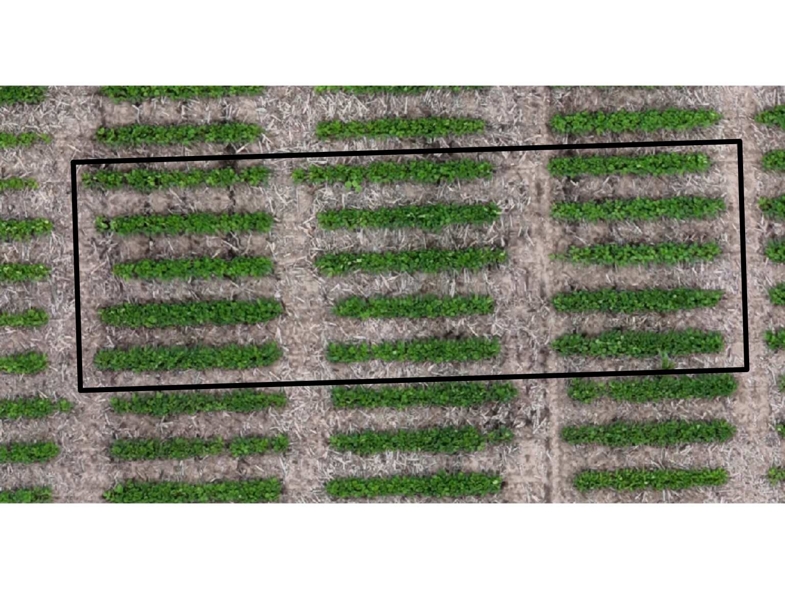
# Create a basemap for further plots
bm <- mosaic_view(mosaic, r = 1, g = 2, b = 3)
#> Warning in CPL_crs_from_input(x): GDAL Message 1: +init=epsg:XXXX syntax is
#> deprecated. It might return a CRS with a non-EPSG compliant axis order. Further
#> messages of this type will be suppressed.
shp <- shapefile_build(
mosaic = mosaic, # the raster file
controlpoints = cpoint, # control points (optional)
basemap = bm, # basemap (optional)
nrow = 5, # number of rows
ncol = 3, # number of columns
layout = "tbrl", # layout definition
serpentine = FALSE # serpentine layout?
)
#> ℹ Building the mosaic✔ Mosaic built [13ms]
#> ℹ Cropping the mosaic✔ Mosaic cropped [425ms]
#> ℹ Creating the shapes✔ Shapes created [143ms]
#> ℹ Finishing the shapefile✔ Shapefile built [49ms]
# see key aspects of the created shapefiles
shapefile_measures(shp)
#> Simple feature collection with 15 features and 11 fields
#> Geometry type: POLYGON
#> Dimension: XY
#> Bounding box: xmin: 734315.6 ymin: 4488975 xmax: 734327 ymax: 4488979
#> Projected CRS: WGS 72BE / UTM zone 14N
#> First 10 features:
#> unique_id block plot_id row column xcoord ycoord area perimeter width
#> 1 1 B01 P0011 1 1 734317.5 4488978 2.943949 9.127652 3.786
#> 2 2 B01 P0012 2 1 734317.5 4488978 2.943949 9.127652 3.786
#> 3 3 B01 P0013 3 1 734317.5 4488977 2.943949 9.127652 3.786
#> 4 4 B01 P0014 4 1 734317.5 4488976 2.943949 9.127652 3.786
#> 5 5 B01 P0015 5 1 734317.6 4488975 2.943949 9.127652 3.786
#> 6 6 B01 P0006 1 2 734321.2 4488978 2.943949 9.127652 3.786
#> 7 7 B01 P0007 2 2 734321.3 4488978 2.943949 9.127652 3.786
#> 8 8 B01 P0008 3 2 734321.3 4488977 2.943949 9.127652 3.786
#> 9 9 B01 P0009 4 2 734321.3 4488976 2.943949 9.127652 3.786
#> 10 10 B01 P0010 5 2 734321.3 4488975 2.943949 9.127652 3.786
#> height geometry
#> 1 0.778 POLYGON ((734315.6 4488979,...
#> 2 0.778 POLYGON ((734315.6 4488978,...
#> 3 0.778 POLYGON ((734315.6 4488977,...
#> 4 0.778 POLYGON ((734315.6 4488976,...
#> 5 0.778 POLYGON ((734315.7 4488976,...
#> 6 0.778 POLYGON ((734319.3 4488979,...
#> 7 0.778 POLYGON ((734319.4 4488978,...
#> 8 0.778 POLYGON ((734319.4 4488977,...
#> 9 0.778 POLYGON ((734319.4 4488976,...
#> 10 0.778 POLYGON ((734319.4 4488976,...The function shapefile_build() returns a Simple Feature
sf object , which is a data structure used to store spatial
objects (points, lines, polygons) along with associated attributes, as
follows:
| Attribute | Description |
|---|---|
| unique_id | A unique identifier for each feature (e.g., plot or area). |
| block | The block grouping of the feature, often used in experimental designs (e.g., “B01” represents Block 1). |
| plot_id | The identifier for the specific plot within the block (e.g., “P0001” represents Plot 1). |
| row | The row number within the plot layout (spatial positioning of the plot within a block). |
| column | The column number within the plot layout (spatial positioning of the plot within a block). |
| geometry | The spatial data representing the polygon boundaries of each feature
POLYGON ((x y, ...)). |
shapefile_build() returns a grid layout that by default
goes from left to right and top to bottom
(layout = "lrtb")
bm + shapefile_view(shp, attribute = "plot_id")By combining the layout and serpentine
arguments, you can generate a total of 16 distinct layouts. The layout
argument controls the primary arrangement of items, while the serpentine
argument introduces an optional serpentine pattern, which alters the
direction of item placement in alternating rows or columns.
The layout argument specifies the orientation of the
layout and is a character string. You can choose from the following
options:
- ‘tblr’: Top to Bottom, Left to Right
- ‘tbrl’: Top to Bottom, Right to Left
- ‘btlr’: Bottom to Top, Left to Right
- ‘btrl’: Bottom to Top, Right to Left
- ‘lrtb’: Left to Right, Top to Bottom
- ‘lrbt’: Left to Right, Bottom to Top
- ‘rltb’: Right to Left, Top to Bottom
- ‘rlbt’: Right to Left, Bottom to Top
The serpentine argument determines whether a serpentine
layout is applied. When set to TRUE, items in alternating
rows or columns will be placed in reverse order, creating a “zig-zag”
pattern. By default, serpentine is set to FALSE, which
means the layout follows the specified direction without altering the
order in alternating rows or columns. Copy and run the following code to
build a Shiny app to demonstrate how these two arguments interact and
affect the layout:
library(shiny)
library(bs4Dash)
library(pliman)
library(leaflet)
# Define the UI
ui <- bs4DashPage(
sidebar = bs4DashSidebar(disable = TRUE),
body = bs4DashBody(
fluidRow(
column(
width = 4, # Controls will be in a 3-column layout
title = "Controls",
selectInput(
inputId = "layout",
label = "Select Layout Orientation:",
choices = c('tblr', 'tbrl', 'btlr', 'btrl', 'lrtb', 'lrbt', 'rltb', 'rlbt'),
selected = 'tblr'
),
checkboxInput(
inputId = "serpentine",
label = "Apply Serpentine Layout?",
value = FALSE
),
numericInput(
inputId = "nrow",
label = "Number of Rows:",
value = 5,
min = 1,
max = 10
),
numericInput(
inputId = "ncol",
label = "Number of Columns:",
value = 3,
min = 1,
max = 10
),
numericInput(
inputId = "pwidth",
label = "Plot width (optional):",
value = NULL,
min = 0,
max = Inf
),
numericInput(
inputId = "pheight",
label = "Plot height (optional):",
value = NULL,
min = 0,
max = Inf
)
),
column(
width = 8, # Map plot will take 9 columns
title = "Map",
leafletOutput("map", height = "640px")
)
)
),
header = bs4DashNavbar(
title = dashboardBrand(
title = "Live demonstration",
color = "white",
opacity = 0.8
),
status = "white",
fixed = TRUE
)
)
# Define the server logic
server <- function(input, output, session) {
url <- "https://github.com/TiagoOlivoto/images/raw/refs/heads/master/pliman/ortho/"
mosaic <- mosaic_input(paste0(url, "orthosmall.tif"), info = FALSE)
cpoint <- shapefile_input(paste0(url, "controlpoints.rds"), info = FALSE)
bm <- mosaic_view(mosaic, r = 1, g = 2, b = 3)
# Build the shapefile
map <- reactive({
if(!is.na(input$pwidth) && !is.na(input$pheight)){
pwidth <- input$pwidth
pheight <- input$pheight
} else{
pwidth <- NULL
pheight <- NULL
}
shp <- shapefile_build(mosaic = mosaic,
controlpoints = cpoint,
basemap = bm,
nrow = input$nrow,
ncol = input$ncol,
layout = input$layout,
serpentine = input$serpentine,
plot_width = pwidth,
plot_height = pheight,
verbose = FALSE)
req(shp)
(bm + shapefile_view(shp, attribute = "plot_id"))@map
})
output$map <- renderLeaflet({
map()
})
}
# Run the application
shinyApp(ui = ui, server = server)Exporting
When working with spatial data in R, two common file formats are
.shp (shapefiles) and .rds (R serialized
files). A shapefile is a standard format in Geographic Information
Systems (GIS) for storing spatial vector data (points, lines, polygons)
and can be imported in any GIS software, like QGIS. Despite the name, a
shapefile is not a single file but a collection of related files:
-
.shp: Contains the geometry (shapes) of the features (points, lines, or polygons). -
.cpg: Contains the character encoding used to interpret the text data in the.dbffile (defaults to UTF-8). -
.shx: An index file that speeds up data access. -
.dbf: Stores the attributes or properties of each feature (like ID, name, etc.). -
.prj: Defines the Coordinate Reference System (CRS), ensuring correct placement on the Earth’s surface.
The .rds file (suggested to work with
pliman) is a format specific to R, used for
saving single R objects (including spatial data) in a serialized form.
It’s ideal for saving R objects in their native format and later loading
them back into R exactly as they were saved.
The function shapefile_export() can be used to export a
shapefile created with shapefile_build() or any other
SpatVector or sf object.
# export to a .rds file
shapefile_export(shp, "shape_rds.rds")
# export to a .shp file
shapefile_export(shp, "shape_shp.shp")Importing shapefiles
You can import previously saved shapefiles using the
shapefile_input() function. This function supports both
.rds files and .shp files, whether they were
exported using shapefile_export() or created in other
software.
However, since all functions in the pliman package are
designed to work with shapefiles generated within pliman,
it’s crucial to ensure that specific fields—such as
unique_id, block, plot_id,
row, and column—are present in the shapefile.
If any of these required fields are missing, unexpected errors may occur
during processing.
shp <- shapefile_input("shape_rds.rds")Exploring the mosaic_analyze() function
mosaic_analyze() is the cornerstone function in pliman
for high-throughput phenotyping. It enables users to
efficiently process orthomosaics and extract a wealth of data from
satellite or drone imagery with just a few lines of code. In most cases,
all you need is an orthomosaic (or even a .jpg image from a
cellphone) and the right function parameters to unlock its full
potential.
Case study
In the example below, mosaic_analyze() is used to count,
measure, and extract image indices at the block, plot, and individual
levels in a lettuce trial. This process is based on an orthomosaic
image, as described in this
paper.
A big thank you to the authors for providing the full-resolution
.tiffile, which enabled me to advance several functionalities in pliman, including high-throughput image analysis and data extraction at multiple levels. This kind of data sharing is invaluable for driving further innovation and tool development.
The trial was conducted using a randomized complete block design with four blocks. The researchers tested the effects of Aspergillus niger application (six different levels, combining both concentration and formulation) and three levels of phosphorus (0%, 50%, 100%) on lettuce growth.

In the plimans shapefile, each plot within the four
blocks is represented by a unique plot_id, such as “P0001,”
“P0002,” etc. These correspond to the following treatments:
| Plot ID | Inoculant | Phosphorus (%) |
|---|---|---|
| P0001 | NI | 0 |
| P0002 | NI | 50 |
| P0003 | NI | 100 |
| P0004 | TS | 0 |
| P0005 | TS | 50 |
| P0006 | TS | 100 |
| P0007 | GR2 | 0 |
| P0008 | GR2 | 50 |
| P0009 | GR2 | 100 |
| P0010 | GR6 | 0 |
| P0011 | GR6 | 50 |
| P0012 | GR6 | 100 |
| P0013 | SC2 | 0 |
| P0014 | SC2 | 50 |
| P0015 | SC2 | 100 |
| P0016 | SC6 | 0 |
| P0017 | SC6 | 50 |
| P0018 | SC6 | 100 |
Importing the needed files
The mosaic_input() function is used to load the mosaic
of a lettuce field, and the shapefile_input() function is
used to load the corresponding shapefile that delineates the plots. You
can also create a shapefile with shapefile_build() (as in
the previous section) or simply define the nrow and
ncol arguments in mosaic_analyze().
In this example, a basemap is created using a mosaic image to serve
as the foundation for further visualizations. While creating a basemap
is not mandatory, it can significantly speed up the process, as
functions like mosaic_analyze(),
shapefile_build(), and shapefile_edit() will
automatically render a leaflet map if one is not provided. By
pre-creating the basemap, you avoid the overhead of rendering multiple
maps, making the workflow more efficient.
Additionally, a shapefile layer is overlaid on top of the basemap to display the levels of the inoculante factor.
url <- "https://github.com/TiagoOlivoto/images/raw/refs/heads/master/pliman/lettuce/"
mos <- mosaic_input(paste0(url, "lettuce.tif"), info = FALSE)
shp <- shapefile_input(paste0(url, "lettuce.rds"), info = FALSE)
# create a basemap
bm <- mosaic_view(mos, r = 1, g = 2, b = 3) # defaults is 1e6.. so here, a bit higher resolution is used
#> ℹ Using `downsample = 2` to match the max_pixels
#> constraint.
bm + shapefile_view(shp, attribute = "p", color_regions = ggplot_color(3))Analyzing the mosaic
There function mosaic_analyze() is all you need now. The
vegetation indexes computed for each plant are defined in the object
indexes. Here, the Normalized Green Red Difference Index
(NGRDI), Green Leaf Index (GLI), and Blue Green Index (BGI) are used.
You can find a list with all build-in vegetation indexes in pliman here.
By setting segment_individuals = TRUE,
mosaic_analyze() shifts its focus to the individual plant
level. Using a threshold-based segmentation method, it isolates each
plant within a plot, enabling precise counting and measurement, provided
that a higher contrast between plant and soi. While the function can
also handle complex backgrounds with additional arguments, that’s not
the focus here. Instead, the power of this approach lies in its ability
to break down each plot into individual components, providing a detailed
analysis of plant morphology, size, and distribution. This transforms
high-throughput phenotyping by moving from a broad plot-level
perspective to an in-depth examination of each plant, unlocking a new
level of precision and insight.
For context, in the original study, the researchers manually measured the diameter of the four central plants in each plot. With
mosaic_analyze(), this process is not only automated but also expanded to include every plant in the plot, providing more comprehensive data in a fraction of the time.
Using segment_index = "GLI", we configure the analysis
to segment soil and identify individual plants based on the GLI index.
The analysis will return both summary statistics for each plot and a map
showing the segmented individual plants.
indexes <- c("NGRDI", "GLI")
an <- mosaic_analyze(
mosaic = mos,
basemap = bm,
r = 1,
g = 2,
b = 3,
shapefile = shp,
plot_index = indexes,
segment_individuals = TRUE,
segment_index = "GLI"
)
#> ── Analyzing the mosaic ──────────────────── Started on 2025-08-23 | 16:08:24 ──
#> ℹ Cropping the mosaic to the shapefile extent...
#> Warning: ! ``segment_plot`` must have length 1 or 4 (the
#> number of drawn polygons).
#> Warning: ! ``segment_individuals`` must have length 1 or 4 (the number of drawn
#> polygons).
#> Warning: ! ``threshold`` must have length 1 or 4 (the
#> number of drawn polygons).
#> Warning: ! ``watershed`` must have length 1 or 4 (the
#> number of drawn polygons).
#> Warning: ! ``segment_index`` must have length 1 or 4
#> (the number of drawn polygons).
#> Warning: ! ``invert`` must have length 1 or 4 (the
#> number of drawn polygons).
#> Warning: ! ``includeopt`` must have length 1 or 4 (the
#> number of drawn polygons).
#> Warning: ! ``opening`` must have length 1 or 4 (the
#> number of drawn polygons).
#> Warning: ! ``closing`` must have length 1 or 4 (the
#> number of drawn polygons).
#> Warning: ! ``filter`` must have length 1 or 4 (the
#> number of drawn polygons).
#> Warning: ! ``erode`` must have length 1 or 4 (the number
#> of drawn polygons).
#> Warning: ! ``dilate`` must have length 1 or 4 (the
#> number of drawn polygons).
#> Warning: ! ``grid`` must have length 1 or 4 (the number
#> of drawn polygons).
#> Warning: ! ``lower_noise`` must have length 1 or 4 (the
#> number of drawn polygons).
#> ✔ Cropping the mosaic to the shapefile extent [1.2s]
#> ℹ Computing vegetation indexes...✔ Computing vegetation indexes [903ms]
#>
#> ── Analyzing block 1 ──
#>
#> ℹ Segmenting individuals within plots...✔ Segmenting individuals within plots [1.6s]
#> ℹ Extracting features from segmented individuals...✔ Extracting features from segmented individuals [171ms]
#> ℹ Extracting plot-level features...✔ Extracting plot-level features [220ms]
#> ℹ Binding the extracted features... ── Analyzing block 2 ──
#> ℹ Binding the extracted features...
#> ℹ Binding the extracted features...✔ Binding the extracted features [74ms]
#> ℹ Segmenting individuals within plots...✔ Segmenting individuals within plots [1.4s]
#> ℹ Extracting features from segmented individuals...✔ Extracting features from segmented individuals [139ms]
#> ℹ Extracting plot-level features...✔ Extracting plot-level features [72ms]
#> ℹ Binding the extracted features... ── Analyzing block 3 ──
#> ℹ Binding the extracted features...
#> ℹ Binding the extracted features...✔ Binding the extracted features [68ms]
#> ℹ Segmenting individuals within plots...✔ Segmenting individuals within plots [1.4s]
#> ℹ Extracting features from segmented individuals...✔ Extracting features from segmented individuals [117ms]
#> ℹ Extracting plot-level features...✔ Extracting plot-level features [67ms]
#> ℹ Binding the extracted features... ── Analyzing block 4 ──
#> ℹ Binding the extracted features...
#> ℹ Binding the extracted features...✔ Binding the extracted features [67ms]
#> ℹ Segmenting individuals within plots...✔ Segmenting individuals within plots [1.1s]
#> ℹ Extracting features from segmented individuals...✔ Extracting features from segmented individuals [132ms]
#> ℹ Extracting plot-level features...✔ Extracting plot-level features [85ms]
#> ℹ Binding the extracted features...✔ Binding the extracted features [18ms]
#> ℹ Summarizing the results... ── Mosaic successfully analyzed ─────────── Finished on 2025-08-23 | 16:08:34 ──
#> ℹ Summarizing the results...✔ Summarizing the results [737ms]Below, you can see the results at the individual plant level. Each
plant within a plot is identified, segmented, and color-coded based on
its measured characteristics (e.g., mean vegetation indices). While you
can use the attribute argument in mosaic_analyze() to
control these visualizations, there’s no need to worry—new plots can
easily be generated after the results are computed, giving you full
flexibility in how the data is displayed.
For each plot, detailed summary statistics are also returned, allowing for in-depth analysis of plant performance across the entire experiment.
an$map_indivWe can gain deeper insights by utilizing the results generated from
mosaic_analyze(). Below, the data is grouped by the
different levels of the inoculante factor to explore how it influences
the analysis.
# see the results averaged by the combination of inoculante and p factors
library(dplyr)
dfino <-
an$result_plot_summ |>
group_by(plot_id, inoculante, p) |>
summarise(across(where(is.numeric), mean))
#> `summarise()` has grouped output by 'plot_id', 'inoculante'. You can override
#> using the `.groups` argument.
# inoculante levels
bm + shapefile_view(dfino, attribute = "inoculante", color_regions = ggplot_color(6))
# phospurus level
bm + shapefile_view(dfino, attribute = "p", color_regions = ggplot_color(3))Vegetation indexes and canopy coverage
This example demonstrates how to use an orthomosaic from a soybean trial to calculate vegetation indexes, specifically the Green Leaf Index (GLI) and the Normalized Green-Red Difference Index (NGRDI). The analysis not only computes these indexes but also segments the plots based on the GLI index, allowing for the remotion of soil effects. Once soil is removed, the canopy coverage within each plot can be computed by the ration between the area covered by plants and the plot area. Here, it is visualized in an interactive map.
The following steps guide you through loading the orthomosaic and corresponding shapefile, calculating vegetation indexes, and visualizing the segmented canopy coverage.
# Define the base URL for the example dataset
url <- "https://github.com/TiagoOlivoto/images/raw/refs/heads/master/pliman/ortho/"
# Load the orthomosaic and shapefile
mosaic <- mosaic_input(paste0(url, "orthomosaic.tif"), info = FALSE)
shp <- shapefile_input(paste0(url, "orthomosaic.rds"), info = FALSE)
# Visualize the mosaic and overlay the shapefile for plot boundaries
bm <- mosaic_view(mosaic, r = 1, g = 2, b = 3) # RGB visualization of the mosaic
#> ℹ Using `downsample = 4` to match the max_pixels
#> constraint.
bm + shapefile_view(shp) # Overlay the shapefile on the mosaic
# Compute the Green Leaf Index (GLI) for the mosaic to highlight vegetation
ind <- mosaic_index(mosaic, index = "GLI", r = 1, g = 2, b = 3)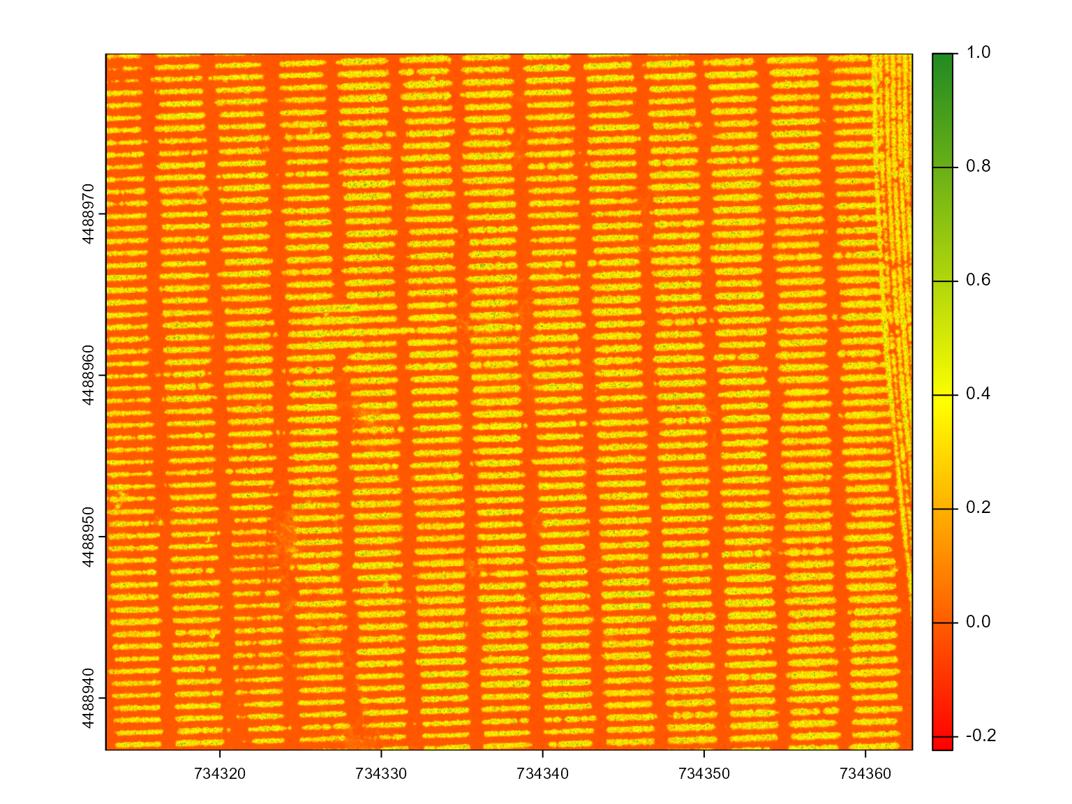
# Segment the mosaic based on the GLI index to distinguish soil and plants
seg <- mosaic_segment(
mosaic = mosaic,
index = "GLI", # Use GLI for segmentation
r = 1, # Red channel
g = 2, # Green channel
b = 3 # Blue channel
)
# Plot the segmented mosaic, showing the separation of plants and soil
mosaic_plot(seg)
# Perform further analysis using mosaic_analyze
# - This calculates both GLI and NGRDI for each plot
# - Segments the plots based on the GLI index
# - Calculates canopy coverage within each plot
res <- mosaic_analyze(
mosaic = mosaic, # The orthomosaic image
shapefile = shp, # The shapefile with plot boundaries
basemap = bm, # Basemap (not mandatory)
plot_index = c("GLI", "NGRDI"), # Vegetation indexes to calculate
segment_plot = TRUE, # Segment plots using the index
segment_index = "GLI", # GLI is used for segmentation
attribute = "coverage" # Calculate canopy coverage
)
#> ── Analyzing the mosaic ──────────────────── Started on 2025-08-23 | 16:09:04 ──
#> ℹ Cropping the mosaic to the shapefile extent...✔ Cropping the mosaic to the shapefile extent [1.9s]
#> ℹ Computing vegetation indexes...✔ Computing vegetation indexes [2.7s]
#>
#> ── Analyzing block 1 ──
#>
#> ℹ Masking vegetation from ground...✔ Vegetation masking completed [4.5s]
#> ℹ Extracting plot-level features...✔ Extracting plot-level features [1.3s]
#> ℹ Binding the extracted features...✔ Binding the extracted features [26ms]
#> ℹ Summarizing the results... ── Mosaic successfully analyzed ─────────── Finished on 2025-08-23 | 16:09:17 ──
#> ℹ Summarizing the results...✔ Summarizing the results [2.3s]
# Display the interactive map showing the plot segmentation
# Color shows the canopy coverage
res$map_plot
# create a plot to shows the NGRDI index
# bm + shapefile_view(res$result_plot, attribute = "mean.NGRDI")Multispectral Indexes
In this example, we use a multispectral orthomosaic to compute
important vegetation indexes such as the Normalized Difference
Vegetation Index (NDVI), Enhanced Vegetation Index (EVI), and Normalized
Difference Red Edge Index (NDRE). You can see a complete
list of multispectral indexes available in pliman for
more details. These indexes are valuable for assessing plant health,
canopy coverage, and other agronomic insights. You can download the
orthomosaic and shapefile to reproduce this analysis by following the
steps below.
The process involves loading the multispectral mosaic and shapefile, calculating the vegetation indexes, and segmenting the plots based on the NDVI index. Additionally, an interactive map will display the segmented plots and canopy coverage metrics.
# Define the base URL for the example dataset
url <- "https://github.com/TiagoOlivoto/images/raw/refs/heads/master/pliman/wheat/"
# Load the orthomosaic and shapefile
mosaic <- mosaic_input(paste0(url, "wheat.tif"), info = FALSE)
shp <- shapefile_input(paste0(url, "wheat.rds"), info = FALSE)
# Generate a basemap
bm <- mosaic_view(mosaic, r = 3, g = 2, b = 1)
#> ℹ Using `downsample = 2` to match the max_pixels
#> constraint.
# - Computes three vegetation indexes: NDVI, EVI, and NDRE
ind <- mosaic_index(
mosaic = mosaic,
index = c("NDVI", "TVI", "NDRE"),
b = 1,
g = 2,
r = 3,
re = 4,
nir = 5,
plot = FALSE
)
#> ── Computing rasters for 3 indices ──────────────────── Started at "16:09:29" ──
#> ■■■■■■■■■■■ 1/3 | ETA: 3s■■■■■■■■■■■■■■■■■■■■■ 2/3 | ETA: 1s■■■■■■■■■■■■■■■■■■■■■■■■■■■■■■■ 3/3 | ETA: 0s
#> ── 3 vegetation indices computed ─────────── Ended at "2025-08-23 | 16:09:33" ──
# NDVI
mosaic_plot(ind[[1]])
shapefile_plot(shp, lwd = 3, add = TRUE)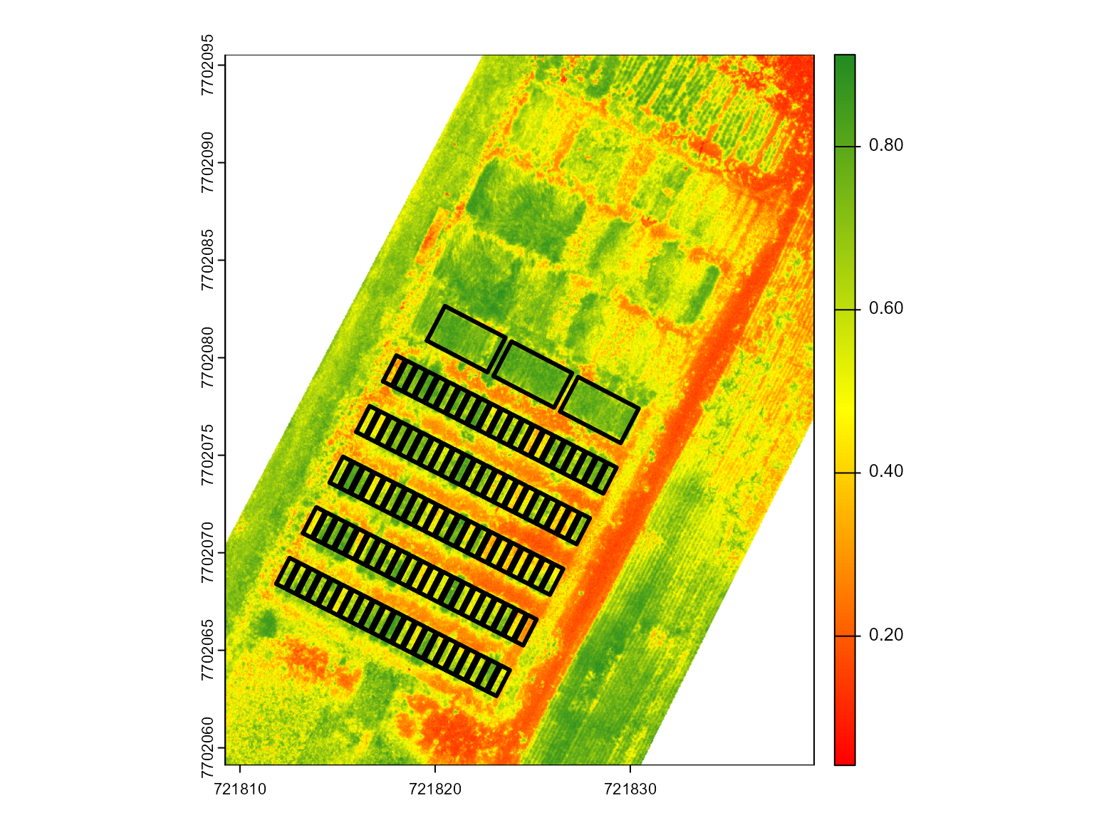
# EVI and NDRE
mosaic_plot(c(ind[[2]], ind[[3]]))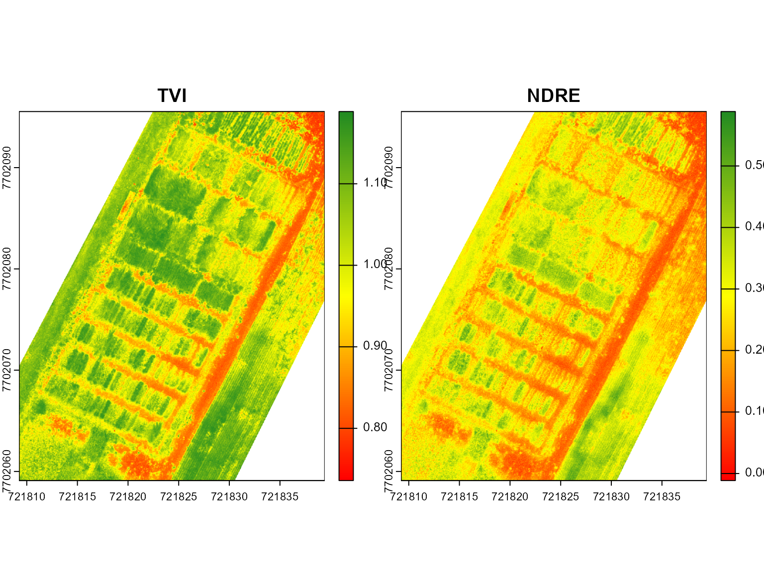
# - Here, I declared the orthomosaic and the bult indexes
# - The basemap will be needed if `plot = TRUE` (default). If not provided, it will be rendered
# - Declare summary statistics
res <- mosaic_analyze(
mosaic = mosaic, # The orthomosaic image
indexes = ind, # we can also declare a raster with computed indexes
basemap = bm, # Use the visualized mosaic as the base map
shapefile = shp, # The shapefile with plot boundaries
summarize_fun = c("min", "median", "max"), # Calculate min, mean, max for the indexes
attribute = "median.NDVI"
)
#> ── Analyzing the mosaic ──────────────────── Started on 2025-08-23 | 16:09:35 ──
#> ℹ Cropping the mosaic to the shapefile extent...
#> Warning: ! ``segment_plot`` must have length 1 or 2 (the
#> number of drawn polygons).
#> Warning: ! ``segment_individuals`` must have length 1 or 2 (the number of drawn
#> polygons).
#> Warning: ! ``threshold`` must have length 1 or 2 (the
#> number of drawn polygons).
#> Warning: ! ``watershed`` must have length 1 or 2 (the
#> number of drawn polygons).
#> Warning: ! ``segment_index`` must have length 1 or 2
#> (the number of drawn polygons).
#> Warning: ! ``invert`` must have length 1 or 2 (the
#> number of drawn polygons).
#> Warning: ! ``includeopt`` must have length 1 or 2 (the
#> number of drawn polygons).
#> Warning: ! ``opening`` must have length 1 or 2 (the
#> number of drawn polygons).
#> Warning: ! ``closing`` must have length 1 or 2 (the
#> number of drawn polygons).
#> Warning: ! ``filter`` must have length 1 or 2 (the
#> number of drawn polygons).
#> Warning: ! ``erode`` must have length 1 or 2 (the number
#> of drawn polygons).
#> Warning: ! ``dilate`` must have length 1 or 2 (the
#> number of drawn polygons).
#> Warning: ! ``grid`` must have length 1 or 2 (the number
#> of drawn polygons).
#> Warning: ! ``lower_noise`` must have length 1 or 2 (the
#> number of drawn polygons).
#> ✔ Cropping the mosaic to the shapefile extent [1.2s]
#>
#> ── Analyzing block 1 ──
#>
#> ℹ Extracting plot-level features...✔ Extracting plot-level features [242ms]
#> ℹ Binding the extracted features... ── Analyzing block 2 ──
#> ℹ Binding the extracted features...
#> ℹ Binding the extracted features...✔ Binding the extracted features [161ms]
#> ℹ Extracting plot-level features...✔ Extracting plot-level features [114ms]
#> ℹ Binding the extracted features...✔ Binding the extracted features [35ms]
#> ℹ Summarizing the results... ── Mosaic successfully analyzed ─────────── Finished on 2025-08-23 | 16:09:37 ──
#> ℹ Summarizing the results...✔ Summarizing the results [202ms]
# Display the interactive map showing the segmented plots
res$map_plotCanopy Height Models
A Canopy Height Model (CHM) represents the height of vegetation or structures above the ground surface, making it a crucial tool for analyzing vegetation structure and biomass. It is derived by subtracting a Digital Terrain Model (DTM), which shows the bare earth surface, from a Digital Surface Model (DSM), which captures the elevation of all surface objects,like plants. By comparing these two models, the CHM provides detailed insights into the height of vegetation, enabling accurate assessments of canopy cover and plant growth in agricultural or forested landscapes.
DSM and DTM are available
# Load DSM, DTM, mask and shapefile
url <- "https://github.com/TiagoOlivoto/images/raw/refs/heads/master/pliman/dsm/"
dsm <- mosaic_input(paste0(paste0(url, "dsm.tif")), info = FALSE)
dtm <- mosaic_input(paste0(paste0(url, "dtm.tif")), info = FALSE)
msk <- mosaic_input(paste0(paste0(url, "mask.tif")), info = FALSE)
shp <- shapefile_input(paste0(paste0(url, "shapefile.rds")), info = FALSE)
# Visualize the DSM and DTM side by side.
# The argument nc = 1 means that the plots will be displayed in a single column.
mosaic_plot(c(dsm, dtm))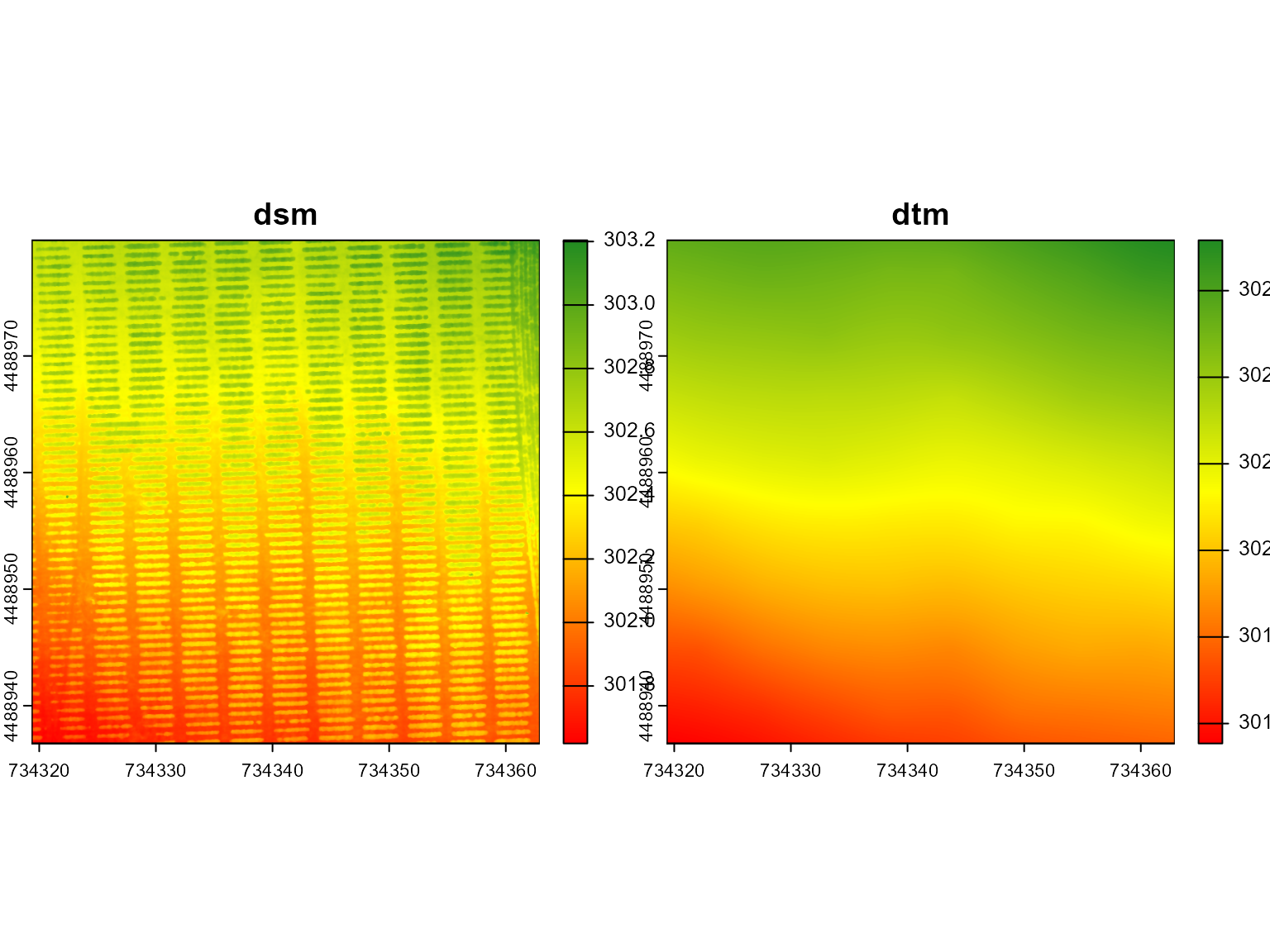
# Compute the Canopy Height Model (CHM) by subtracting the DTM from the DSM.
# The `mask` parameter specifies the regions to be used, and `mask_soil = FALSE`
# means that areas identified by the mask are considered non-soil (i.e., representing the plants).
res <- mosaic_chm(dsm = dsm,
dtm = dtm,
mask = msk,
mask_soil = FALSE)
#> ── Canopy Height-Model generation ─────────────────── "2025-08-23 | 16:09:48" ──
#> ℹ Building the canopy height model...✔ Building the canopy height model [1.8s]
# Extract canopy height values from the CHM using the provided shapefile.
# This will associate the height values with the polygons in the shapefile.
chmvals <- mosaic_chm_extract(res, shp)
# Visualize the DSM with a custom color palette to represent different elevation levels.
pal <- custom_palette(c("#8B4513", "#B2DF8A", "forestgreen"), n = 10)
bm <- mosaic_view(dsm, color_regions = pal)
#> ℹ Using `downsample = 2` to match the max_pixels constraint.
#> Number of pixels is above 1e+06.Only about 1e+06 pixels will be shown.
#> You can increase the value of `maxpixels` to 1000980 to avoid this.
# Overlay the shapefile on top of the DSM visualization, using the "coverage" attribute
# from the shapefile to define the regions of interest.
bm + shapefile_view(chmvals, attribute = "coverage")Building DTM from DSM
In field experiments, the Digital Terrain Model (DTM) is frequently
obtained before sowing and represents the bare soil. But, if we could
derivate DTM from DSM? If a DTM is not provided,
mosaic_chm() will derive DTM from DSM using an
interpolation strategy.
# Interpolate DTM using a moving window
res2 <- mosaic_chm(
dsm,
mask = msk,
window_size = c(4, 4),
mask_soil = FALSE
)
#> ── Canopy Height-Model generation ─────────────────── "2025-08-23 | 16:09:58" ──
#> ℹ Extracting ground points for each moving window...✔ Extracting ground points for each moving window [1.5s]
#> ℹ Interpolating ground points...✔ Interpolating ground points [3.1s]
#> ℹ Resampling and masking the interpolated raster...✔ Resampling and masking the interpolated raster [1.3s]
#> ℹ Building the canopy height model...✔ Building the canopy height model [1.1s]
# Extract CHM values
chmvals2 <- mosaic_chm_extract(res2, shp)
# Quantile 95
bm + shapefile_view(chmvals2, attribute = "q95")
# Entropy
# bm + shapefile_view(chmvals2, attribute = "entropy")Counting and measuring distance between plants
In this example, we use an RGB orthomosaic from a potato field to
analyze and segment individual plants within the plots. The analysis
involves loading the mosaic and corresponding shapefile, cropping the
mosaic to the area defined by the shapefile, and then segmenting
individual plants using a custom vegetation index. When
map_individuals = TRUE is used, important metrics such as
the average distance between plants and the coefficient of variation for
each cropping row are also computed.
# Download and load orthomosaic and shapefile
url <- "https://github.com/TiagoOlivoto/images/raw/refs/heads/master/pliman/potato/"
mos <- mosaic_input(paste0(url, "potato.tif"))
shp <- shapefile_input(paste0(url, "potato.rds"))
bm <- mosaic_view(mos)
res <-
mosaic_analyze(
mosaic = mos,
basemap = bm,
shapefile = shp,
plot_index = "GLI",
segment_individuals = TRUE,
map_individuals = TRUE,
map_direction = "horizontal", # default
attribute = "cv"
)
pal <- c( "#fde725", "#5ec962", "#21918c", "#3b528b", "#440154")
p1 <- shapefile_view(res$result_plot_summ, attribute = "cv", color_regions = pal)
p2 <- shapefile_view(res$result_indiv, type = "centroid", attribute = "area")
(bm + p1) | p2The interactive map above shows the segmented potato plants within
each row. Note that some plots were not rendered due to the absence of
identified plants. It is important to highlight the structure of the
res object:
names(res)When map_individuals = TRUE is used, the
result_individ_map object contains the distances between
each plant within the plots. By default, the mapping occurs in the
horizontal direction.
res[["result_individ_map"]][["distances"]][["B01_P0001"]]The objects means and cvs hold the average
distances and coefficients of variation, respectively.
library(patchwork)
pmean <-
ggplot(res$result_plot_summ, aes(x = mean_distance)) +
geom_histogram() +
labs(x = "Average distance between plants",
y = "Number of plots")
pcv <-
ggplot(res$result_plot_summ, aes(x = cv)) +
geom_histogram(bins = 10) +
labs(x = "Coefficient of variation (%)",
y = "Number of plots")
pmean + pcvBelow, we’ll explore two contrasting plots to demonstrate how this information can be valuable for assessing plot uniformity.
library(dplyr)
par(mfrow = c(2, 1))
p1 <-
res$result_indiv |>
filter(plot_id == "P0184")
# plot
p1plot <-
res$result_plot_summ |>
filter(plot_id == "P0184")
plot1 <- mosaic_crop(mos, shapefile = p1plot, buffer = 0.2)
coords <- p1[, c("x", "y")] |> sf::st_drop_geometry() |> arrange(x)
mosaic_plot_rgb(plot1, main = "P0184: Average distance: 0.243 m; CV: 14.1%")
lines(coords, lwd = 2)
shapefile_plot(p1plot, add = TRUE, border = "blue", lwd = 3)
points(p1$x, p1$y, pch = 16, cex = 2, col = "red")
p2 <-
res$result_indiv |>
filter(plot_id == "P0204")
p2plot <-
res$result_plot_summ |>
filter(plot_id == "P0204")
plot2 <- mosaic_crop(mos, shapefile = p2plot, buffer = 0.2)
coords2 <- p2[, c("x", "y")] |> sf::st_drop_geometry() |> arrange(x)
mosaic_plot_rgb(plot2, main = "P0204: Average distance: 0.325 m; CV: 64.0%")
lines(coords2, lwd = 2)
shapefile_plot(p2plot, add = TRUE, border = "blue", lwd = 3)
points(p2$x, p2$y, pch = 16, cex = 2, col = "red")Handling complex backgrounds
Challenges
Threshold-based methods often struggle with complex backgrounds typical of field experiments, where diverse soil types, colors, and textures introduce considerable variability. This variability reduces the contrast between plants and soil, complicating the computation of vegetation indexes in orthomosaics. When soil and plant pixels have similar reflectance values, thresholding fails to separate them accurately, leading to erroneous plant segmentation, which in turn affects vegetation index calculations, plant measurements, and analytical outputs.
For instance, in this section, we use an orthomosaic from a field with complex soil backgrounds, generously provided by Lucas Côrredo-UFV, to illustrate the limitations of threshold-based segmentation and how they can be overcome using simple alternatives that are not based on complex machine learning-based methods.
url <- "https://github.com/TiagoOlivoto/images/raw/refs/heads/master/pliman/citrus/"
mosaic <- mosaic_input(paste0(url, "citrus_mos.tif"), info = FALSE)
shp <- shapefile_input(paste0(url, "citrus_shp.rds"), info = FALSE)
bm <- mosaic_view(mosaic, r = 1, g = 2, b = 3, max_pixels = 5e6)
#> ℹ The number of pixels is very high, which might slow the rendering process.
#> ℹ Using `downsample = 3` to match the max_pixels constraint.
bmIf you take a closer look at the orthomosaic, you’ll notice that the soil background is complex, with varying colors and textures that make it challenging to separate from the plants. This complexity poses a significant challenge for threshold-based segmentation methods, which rely on clear distinctions between plants and soil to accurately identify and measure vegetation indexes. Early in this material we’ve seen that the GLI index is a good option to segment plants from soil. However, in this case, segmentation using threshold-based methods may not be effective due to the complex background.
seg <- mosaic_segment(mosaic, index = "GLI", r = 1, g = 2, b = 3)
mosaic_plot(seg)The segmentation results indicate that the threshold-based method struggles to distinguish plants from soil, resulting in inaccurate plant identification and measurements. This challenge highlights the need for alternative methods capable of handling complex backgrounds more effectively.
When vegetation indexes are insufficient
Threshold-based methods often fail to distinguish plants from soil, making it necessary to explore strategies beyond vegetation indexes. A more robust approach involves using machine learning, particularly deep learning models, to enhance plant segmentation and analysis in orthomosaics. These models can identify intricate patterns and features, offering superior differentiation between plants and soil compared to traditional methods. However, such models have not yet been integrated into pliman 3.0. So, how can we enhance segmentation with simpler approaches? The solution lies in leveraging a 3D perspective with a Canopy Height Model (CHM).
Do we really need AI-based models?
To improve plant segmentation, incorporating a digital surface model
(DSM) can be highly effective, as it provides valuable height
information for objects within the orthomosaic. The
mosaic_chm_mask() function allows generating a mask from a
Canopy Height Model (CHM) derived using the mosaic_chm()
function. This mask enables segmentation based on plant height instead
of relying solely on color, which can more precisely distinguish plants
from soil, particularly in complex backgrounds. This method offers a
straightforward, non-AI solution for overcoming segmentation challenges,
delivering enhanced plant isolation without the need for machine
learning algorithms, mainly for examples like this, where the orange
trees are relatively tall, facilitating the separation between plants
and soil.
dsm <- mosaic_input(paste0(url, "citrus_dsm.tif"), info = FALSE)
# create a mask, retaining only pixels between 1 and 5 meters
mask <- mosaic_chm_mask(
dsm = dsm,
window_size = c(3, 3), # Window size for interpolating the DTM
lower = 0.5, # Lower limit for the mask (height)
upper = 3 # Upper limit for the mask (height)
)
mosaic_plot(mask)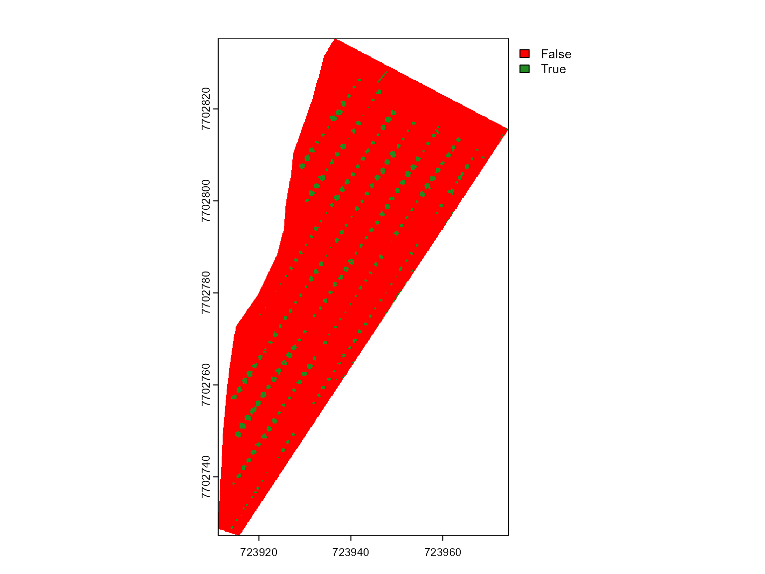
Great advance! Now, we have a mask that retains only pixels between
0.5 and 3 meters in height, effectively isolating the plants from the
soil. This mask can be now used in mosaic_analyze() to
segment the plants and calculate vegetation indexes more accurately.
# Analyze the segmented mosaic data
mos <- mosaic_analyze(
mosaic = mosaic, # The input mosaic
basemap = bm, # The basemap for visualization.
r = 1, g = 2, b = 3, # Specify the red, green, and blue channels
mask = mask, # Apply the mask created previously
# dsm = dsm, # or directly use the DSM
# dsm_lower = 0.5, # or directly use the DSM
# dsm_upper = 3, # or directly use the DSM
#dsm_window_size = c(3, 3) # or directly use the DSM
shapefile = shp, # Shapefile to outline regions of interest
segment_individuals = TRUE, # Enable segmentation
plot_index = c("NGRDI", "GLI"), # Vegetation indexes to compute for each plant
lower_noise = 0, # Avoid removing small plants
filter = 10, # Size of the filter applied to reduce noise
watershed = FALSE # Disable watershed algorithm
)
#> ── Analyzing the mosaic ──────────────────── Started on 2025-08-23 | 16:11:01 ──
#> ℹ Cropping the mosaic to the shapefile extent...✔ Cropping the mosaic to the shapefile extent [26ms]
#> ℹ Computing vegetation indexes...✔ Computing vegetation indexes [9.9s]
#>
#> ── Analyzing block 1 ──
#>
#> ℹ Segmenting individuals...✔ Segmenting individuals [20.1s]
#> ℹ Extracting plant-level features...✔ Extracting plant-level features [2.2s]
#> ℹ Extracting plot-level features...✔ Extracting plot-level features [1.9s]
#> ℹ Binding the extracted features...✔ Binding the extracted features [16ms]
#> ℹ Summarizing the results... ── Mosaic successfully analyzed ─────────── Finished on 2025-08-23 | 16:11:38 ──
#> ℹ Summarizing the results...✔ Summarizing the results [2s]
# Summary
mos$result_plot_summ
#> Simple feature collection with 1 feature and 18 fields
#> Geometry type: POLYGON
#> Dimension: XY
#> Bounding box: xmin: 723911.2 ymin: 7702727 xmax: 723974.3 ymax: 7702835
#> Projected CRS: WGS 84 / UTM zone 23S
#> # A tibble: 1 × 19
#> block plot_id row column n area_sum area coverage perimeter length
#> <chr> <chr> <dbl> <dbl> <dbl> <dbl> <dbl> <dbl> <dbl> <dbl>
#> 1 B01 P0001 1 1 223 4120. 18.5 1.46 5.47 1.43
#> # ℹ 9 more variables: width <dbl>, diam_min <dbl>, diam_mean <dbl>,
#> # diam_max <dbl>, mean.NGRDI <dbl>, mean.GLI <dbl>, individual <chr>,
#> # plot_area [m^2], geometry <POLYGON [m]>The identified plants are displayed on the map, color-coded by their mean NGRDI (Normalized Green-Red Difference Index) values. Thias visualization highlights plant distribution and relative health across the field, making it easier to identify variations in vegetation index values and assess plant vigor.
bm +
shapefile_view(mos$result_indiv[-1, ],
attribute = "diam_mean",
alpha.regions = 0.6)The results show that the CHM-based segmentation method effectively isolates plants from the soil, providing accurate plant identification and measurements. This approach offers a simple yet powerful alternative to threshold-based methods, demonstrating the value of leveraging 3D information to enhance plant segmentation in orthomosaics.
Below, we explore the individual plant data to gain deeper insights into plant health across the field.
coords <- shapefile_measures(mos$result_indiv[-1, ])
model <- shapefile_interpolate(coords, z = "mean.NGRDI")
mosaic_plot_rgb(mosaic)Vectorizing field masks
In this section, we use another orthomosaic from citrus field provided by Lucas Côrredo-UFV. This dataset includes both RGB and multispectral indices, as well as a mask derived from the digital surface model, enhancing our ability to differentiate features in the field.
url <- "https://github.com/TiagoOlivoto/images/raw/refs/heads/master/pliman/multispec/"
rgb <- mosaic_input(paste0(url, "citrus_rgb.tif"), info = FALSE)
mes <- mosaic_input(paste0(url, "citrus_ms.tif"), info = FALSE)
mask <- mosaic_input(paste0(url, "citrus_mask.tif"), info = FALSE)
mosaic_plot_rgb(rgb)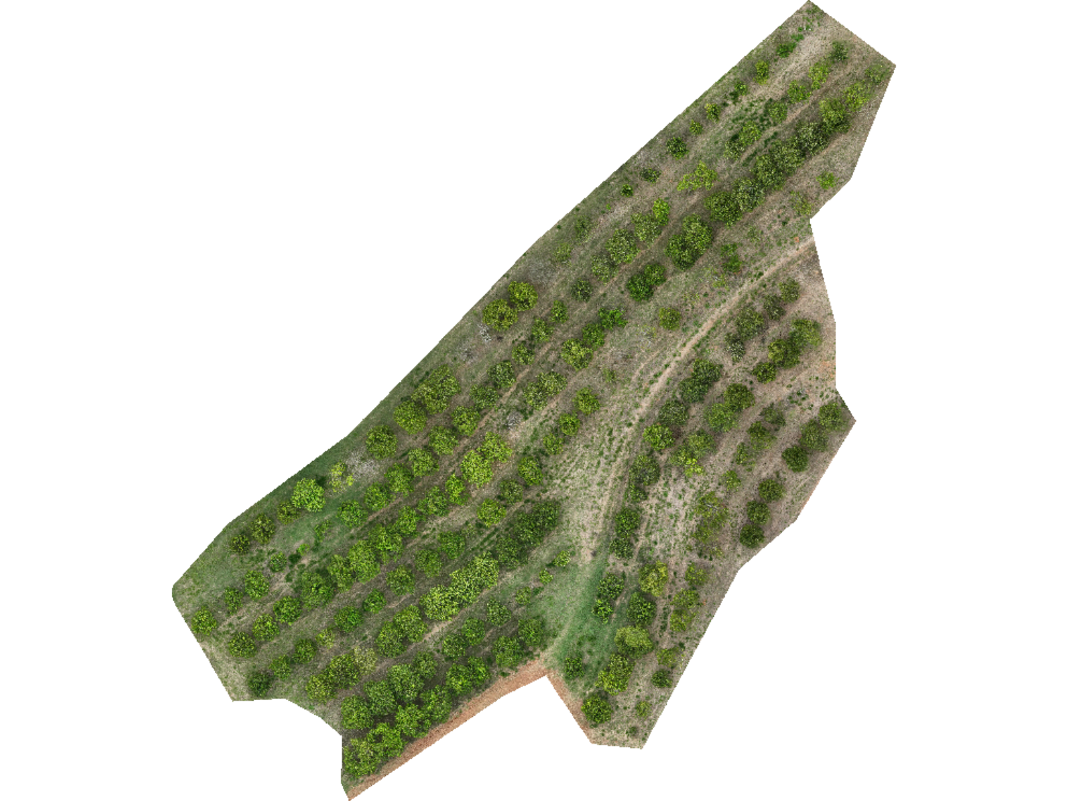
mosaic_plot(mask)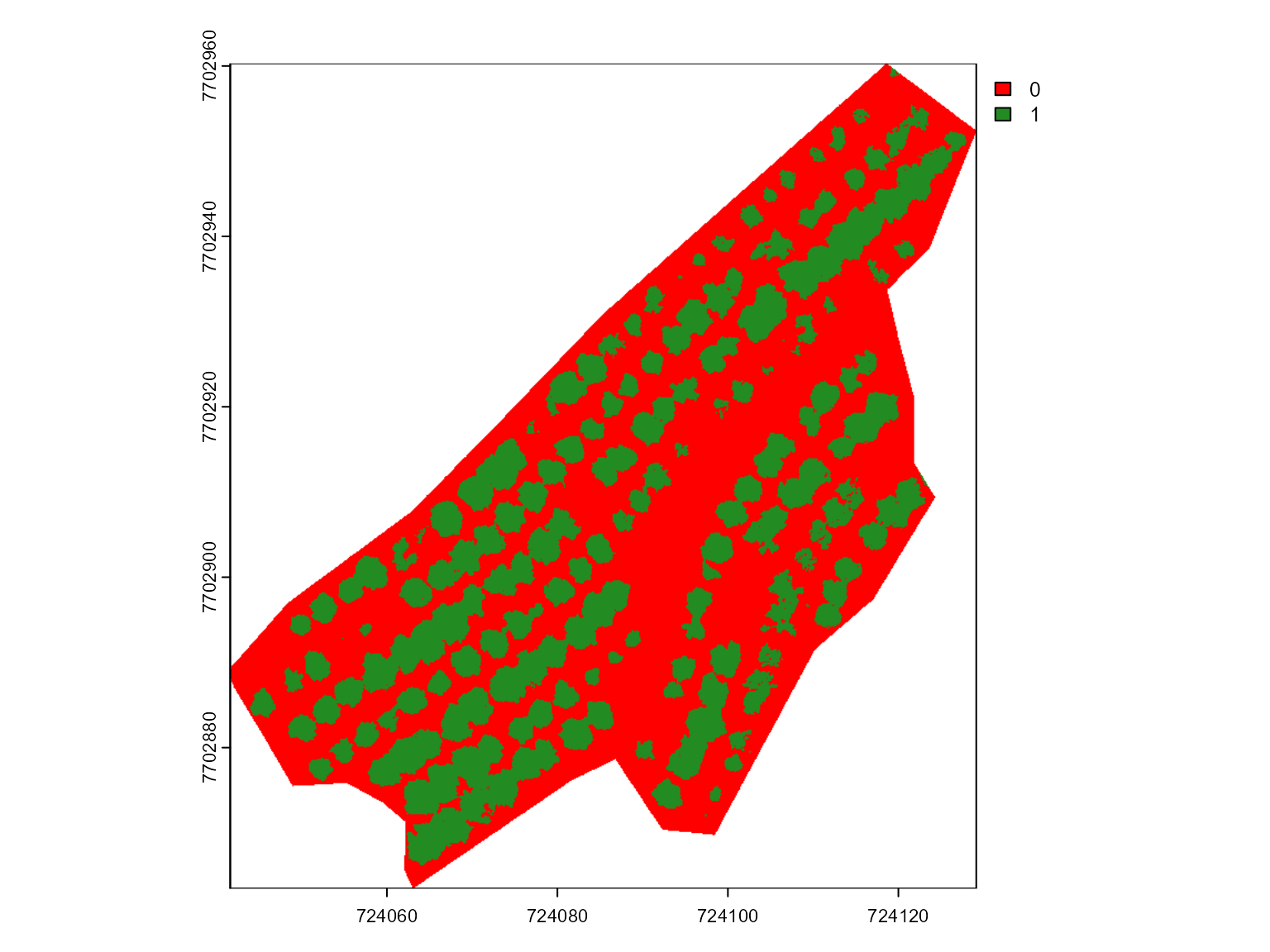
In this section, we take a different approach from the previous
example, using the mask file to create an sf object that allows
vegetation index extraction at the individual level. Specifically, we
will vectorize the raster mask using the mosaic_vectorize()
function.
The mosaic_vectorize() function converts a raster mask
(SpatRaster object) into a vectorized sf
object, with customizable options for morphological operations and
filtering to enhance object detection and segmentation. The function
includes an option for watershed segmentation, which, if enabled,
applies watershed-based segmentation to distinguish touching objects,
like the needed in this case.
Morphological operations (opening, closing,
filter, erode, dilate) allow
further customization, helping to refine the mask by removing noise,
filling small gaps, or smoothing object edges. The
lower_size and upper_size arguments allow
size-based filtering, while topn_lower and
topn_upper select objects based on their area.
Through these settings, mosaic_vectorize() enables
vectorization tailored to individual vegetation elements, optimizing
extraction of vegetation indices at the plant level. Let’s vectorize the
binary mask using filter = 10 to remove some noises and
erode = 10 to erode 10 pixels from the edges of each object
to avoid edge effects
bm <- mosaic_view(rgb, r = 1, g = 2, b = 3)
#> ℹ Using `downsample = 3` to match the max_pixels
#> constraint.
# Vectorize the shapefile
shp <- mosaic_vectorize(mask,
filter = 10,
erode = 15)
bm + shapefile_view(shp)With the shapefile representing individual plants, we can now extract
vegetation indices at the plant level. Instead of applying
mosaic_analyze(), we’ll use mosaic_index() to
compute specific multispectral indices.
vind <-
mosaic_index(mes,
index = c("RDVI", "NDVI"),
b = 1,
r = 2,
nir = 3,
re = 4,
g = NA)
#> ── Computing rasters for 2 indices ──────────────────── Started at "16:11:58" ──
#> ■■■■■■■■■■■■■■■■ 1/2 | ETA: 1s■■■■■■■■■■■■■■■■■■■■■■■■■■■■■■■ 2/2 | ETA: 0s
#> ── 2 vegetation indices computed ─────────── Ended at "2025-08-23 | 16:12:01" ──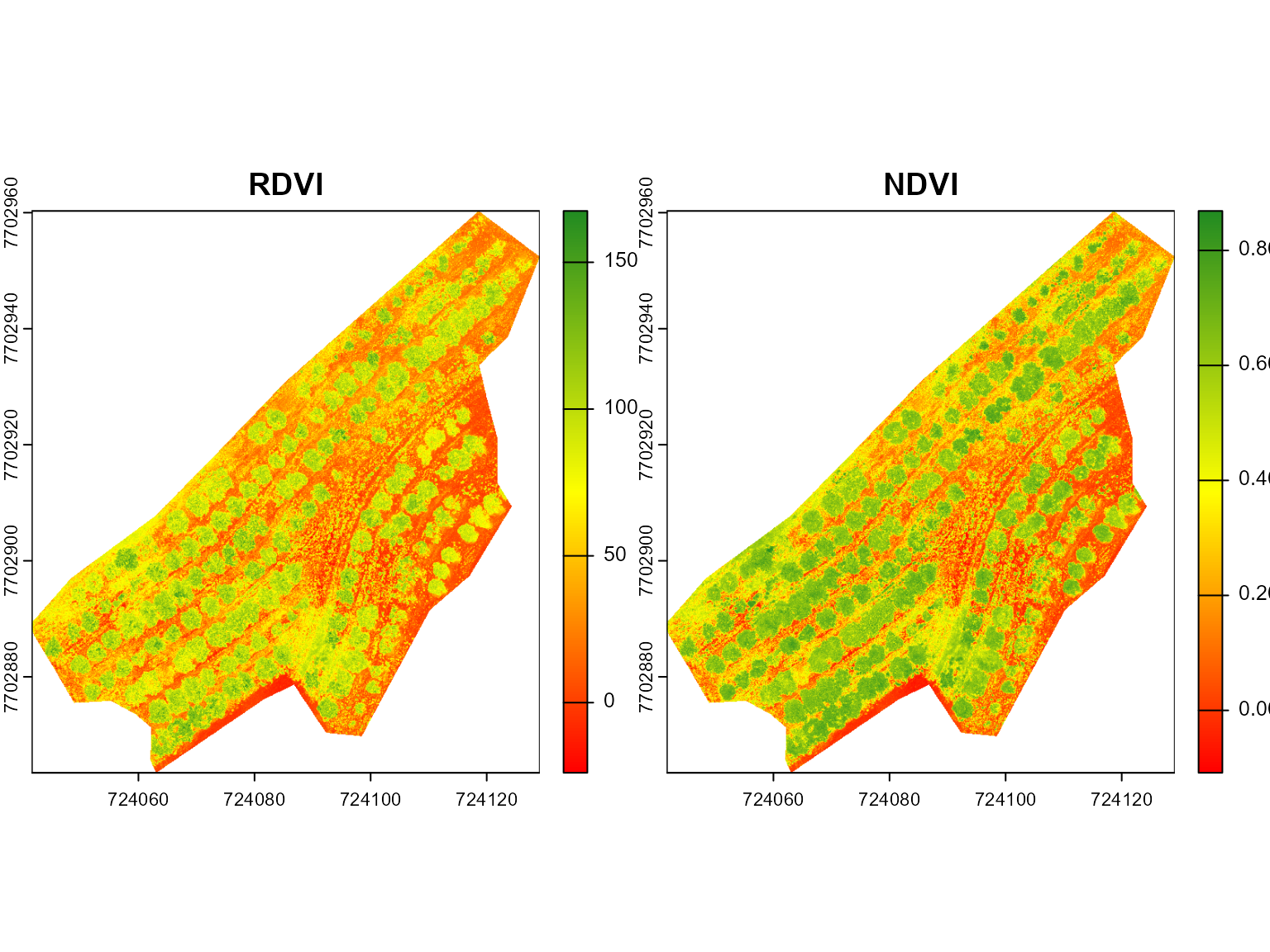
results <- mosaic_extract(vind, shp)
#> | | | 0% | | | 1% | |= | 1% | |= | 2% | |== | 3% | |=== | 4% | |=== | 5% | |==== | 5% | |==== | 6% | |===== | 7% | |====== | 8% | |====== | 9% | |======= | 10% | |======= | 11% | |======== | 11% | |======== | 12% | |========= | 12% | |========= | 13% | |========== | 14% | |========== | 15% | |=========== | 15% | |=========== | 16% | |============ | 16% | |============ | 17% | |============ | 18% | |============= | 18% | |============= | 19% | |============== | 20% | |=============== | 21% | |=============== | 22% | |================ | 22% | |================ | 23% | |================= | 24% | |================== | 25% | |================== | 26% | |=================== | 27% | |=================== | 28% | |==================== | 28% | |==================== | 29% | |===================== | 30% | |====================== | 31% | |====================== | 32% | |======================= | 32% | |======================= | 33% | |======================= | 34% | |======================== | 34% | |======================== | 35% | |========================= | 35% | |========================= | 36% | |========================== | 37% | |========================== | 38% | |=========================== | 38% | |=========================== | 39% | |============================ | 39% | |============================ | 40% | |============================= | 41% | |============================= | 42% | |============================== | 43% | |=============================== | 44% | |=============================== | 45% | |================================ | 45% | |================================ | 46% | |================================= | 47% | |================================== | 48% | |================================== | 49% | |=================================== | 49% | |=================================== | 50% | |=================================== | 51% | |==================================== | 51% | |==================================== | 52% | |===================================== | 53% | |====================================== | 54% | |====================================== | 55% | |======================================= | 55% | |======================================= | 56% | |======================================== | 57% | |========================================= | 58% | |========================================= | 59% | |========================================== | 60% | |========================================== | 61% | |=========================================== | 61% | |=========================================== | 62% | |============================================ | 62% | |============================================ | 63% | |============================================= | 64% | |============================================= | 65% | |============================================== | 65% | |============================================== | 66% | |=============================================== | 66% | |=============================================== | 67% | |=============================================== | 68% | |================================================ | 68% | |================================================ | 69% | |================================================= | 70% | |================================================== | 71% | |================================================== | 72% | |=================================================== | 72% | |=================================================== | 73% | |==================================================== | 74% | |==================================================== | 75% | |===================================================== | 76% | |====================================================== | 77% | |====================================================== | 78% | |======================================================= | 78% | |======================================================= | 79% | |======================================================== | 80% | |========================================================= | 81% | |========================================================= | 82% | |========================================================== | 82% | |========================================================== | 83% | |========================================================== | 84% | |=========================================================== | 84% | |=========================================================== | 85% | |============================================================ | 85% | |============================================================ | 86% | |============================================================= | 87% | |============================================================= | 88% | |============================================================== | 88% | |============================================================== | 89% | |=============================================================== | 89% | |=============================================================== | 90% | |================================================================ | 91% | |================================================================ | 92% | |================================================================= | 93% | |================================================================== | 94% | |================================================================== | 95% | |=================================================================== | 95% | |=================================================================== | 96% | |==================================================================== | 97% | |===================================================================== | 98% | |===================================================================== | 99% | |======================================================================| 99% | |======================================================================| 100%
# overlay the shapefile to the basemap
bm + shapefile_view(
results,
attribute = "median.NDVI"
)